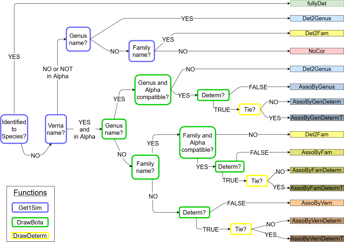
Method of association of a vernacular name with a botanical name
Be a tree t with a vernacular name v. This tree can have a known genus, only a known family or no botanical information at all. The associated botanical names follow a categorical distribution \(\mathcal{Cat} (\alpha^v)\) where \(\alpha^v = [\alpha^v_1, \alpha^v_2,..., \alpha^v_N]\) is the vector of probability of association of between the vernacular name v and each botanical name (so \(\sum_{s=1}^N \alpha^v_i =1)\)) and N is the number of botanical name present in the inventories taken as a reference and/or the prior knowledge.
To get the vector \(\alpha^v\), we use a Dirichlet-categorical scheme to combine a prior information based on expert knowledge that we updated with observed frequencies of association between the vernacular name v and each botanical name in the reference inventories \(f^v = [f^v_1, f^v_2,..., f^v_N]\) (Aubry-Kientz et al. 2013).
We consider \(\lambda^v\) as hyperparameters of \(\alpha^v\), i.e. the parameters of the prior distribution of \(\alpha^v\). The prior probability of association of the vernacular v with each botanical name s in [1,N] is \(\lambda^v_s\) and is obtained as follows:
- \(\lambda^v_s = \frac{1}{m_v}\) if the botanical name s is associated to the vernacular name v AND belongs to the same genus than t (if there is a know genus) and the same family than t (if there is a known family). \(m_v\) is the number of botanical names meeting these conditions.
- \(\lambda^v_s = \frac{\epsilon}{N-m_v}\) otherwise (\(\epsilon\) being a background noise)
The prior distribution of \(\alpha^v \sim \mathcal{Dir}(N, \lambda^v)\).
As the Dirichlet distribution is the conjugated prior of the categorical distribution, the posterior distribution of the probabilities of associations \(\alpha^v\) can be obtained by updating the expert knowledge with the observed frequency of association \(f^v\).
So the posterior distribution of probability of association is \(\alpha^v | f^v,\lambda^v \sim \mathcal{Dir} (N, w_p \times \lambda^v_1 + (1-w_p) \times f^v_1,...,w_p \times \lambda^v_N+(1-w_p) \times f^v_N)\) where \(w_p\) is the weight given to the prior information.
NB: \(\lambda^v\) and \(f^v\) are taken as frequencies to give the same weight to give the same weight to the prior and the observations when given an equal weight (i.e. when \(w_p=0.5\)).
In practice, as we don’t want to calculate the vector \(\alpha^v\) for each tree, we create a matrix \(\alpha\) of \(\alpha^v\) that will be used for all trees. We therefore don’t have any information on the family or the genus at this stage. We take \(\lambda^v_s = 0\) for the botanical names that are not associated to the vernacular name v according to expert knowledge. The matrix \(\alpha\) have a lot of 0 (in case when there is no association according to expert knowledge, nor according to the data). When we then consider the tree t, we replace non-null values by 0 when botanical names don’t belong to the same genus than t (if there is a known genus) and the same family than t (if there is a known family). We then replace 0 by \(\epsilon\) divided by the number of value=0.
Bibliography
Aubry-Kientz, Mélaine, Bruno Hérault, Charles Ayotte-Trépanier, Christopher Baraloto, and Vivien Rossi. 2013. “Toward Trait-Based Mortality Models for Tropical Forests.” Edited by Francesco de Bello. PLoS ONE 8 (5): e63678. https://doi.org/10.1371/journal.pone.0063678.
